Revenue Predictor Model
The basics of machine learning.
July, 2025
Introduction
Machine learning is extremely approachable these days, with many libraries and frameworks that make it easy to create a model. I had never done any machine learning before, so I wanted to try it out.
This is an in-depth article of how to create a basic model, so it is quite lengthy.
Dataset and Tools
Kaggle is a great resource for datasets. I found a datasets with purchases, categories, and customer traits by Vineet Bahl. Click here to find the dataset . I stored my raw CSV in the data/raw folder.
In specific, here were all the columns in the dataset:
- Date: Date of the sale. (Date)
- Year: Year of the sale. (Integer)
- Month: Month of the sale. (Integer)
- Customer Age: Age of the customer. (Integer)
- Customer Gender: Gender of the customer. (String)
- Country: Country of the customer. (String)
- State: State of the customer. (String)
- Product Category: Category of the product. (String)
- Sub Category: Sub-category of the product. (String)
- Quantity: Quantity of the product sold/purchased. (Integer)
- Unit Cost: Cost of the product per unit. (Float)
- Unit Price: Price of the product per unit. (Float)
- Revenue: Total revenue generated from the sale. (Float)
- Column1: Unknown. (Unknown)
As for what tools I decided to use, I chose Python and specifically Jupiter Notebooks for creating the model. It was easy to use and the notebook approach made it modular and dynamic in terms of testing and iterating on the model. Some python packages include Pandas for data, Scikit-Learn for the model, and MatPlotLib and Seaborn for graphs.
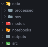
If you are following along, here is my folder structure:
Creating a model takes 4 steps: Exploratory Data Analysis, Data Preprocessing, Model Creation, and Model Evaluation.
Exploratory Data Analysis
Before creating a model, it is important to understand the data. This is done through Exploratory Data Analysis (EDA). EDA is the process of analyzing your dataset visually and statistically to understand its structure, patterns, and anomalies before doing any modeling or machine learning.
Our goal is to:
- Understand what your data looks like
- Identify potential errors or missing values.
- Find relationships between variables (e.g., age vs. revenue).
- Get ideas for feature engineering.
- Check if your data meets assumptions for modeling.
After downloading the dataset as a CSV and putting it in the data/raw folder, we can start to look at it by importing it into a Pandas DataFrame. I created a file called 01_eda.ipynb in the notebooks folder.
I import Pandas and read the CSV into a dataframe, which is basically a 2D data structure similar to a matrix.
import pandas as pd
db = pd.read_csv("../data/raw/SalesForCourse_quizz_table.csv")
If we read the headers, we get:
print(db.head(5))index Date Year Month Customer Age Customer Gender
0 0 02/19/16 2016.0 February 29.0 F
1 1 02/20/16 2016.0 February 29.0 F
2 2 02/27/16 2016.0 February 29.0 F
3 3 03/12/16 2016.0 March 29.0 F
4 4 03/12/16 2016.0 March 29.0 F
Country State Product Category Sub Category Quantity
0 United States Washington Accessories Tires and Tubes 1.0
1 United States Washington Clothing Gloves 2.0
2 United States Washington Accessories Tires and Tubes 3.0
3 United States Washington Accessories Tires and Tubes 2.0
4 United States Washington Accessories Tires and Tubes 3.0
Unit Cost Unit Price Cost Revenue Column1
0 80.00 109.000000 80.0 109.0 NaN
1 24.50 28.500000 49.0 57.0 NaN
2 3.67 5.000000 11.0 15.0 NaN
3 87.50 116.500000 175.0 233.0 NaN
4 35.00 41.666667 105.0 125.0 NaN We can see all columns in the dataset, along with the first 5 rows of data. Note that the last column seems to have all NaN.
Reading the dataframe's info gets us:
print(db.info())<class 'pandas.core.frame.DataFrame'> RangeIndex: 34867 entries, 0 to 34866 Data columns (total 16 columns): # Column Non-Null Count Dtype --- ------ -------------- ----- 0 index 34867 non-null int64 1 Date 34866 non-null object 2 Year 34866 non-null float64 3 Month 34866 non-null object 4 Customer Age 34866 non-null float64 5 Customer Gender 34866 non-null object 6 Country 34866 non-null object 7 State 34866 non-null object 8 Product Category 34866 non-null object 9 Sub Category 34866 non-null object 10 Quantity 34866 non-null float64 11 Unit Cost 34866 non-null float64 12 Unit Price 34866 non-null float64 13 Cost 34866 non-null float64 14 Revenue 34867 non-null float64 15 Column1 2574 non-null float64 dtypes: float64(8), int64(1), object(7) memory usage: 4.3+ MB None
We can see that column 15, called "Column1", has a much smaller Non-Null count compared to all other columns. Also seen is the data type that each column uses.
Can we find any outliers? Let's take a high level visual look first at age.
import matplotlib.pyplot as plt
import seaborn as sns

sns.boxplot(data=db, x='Customer Age')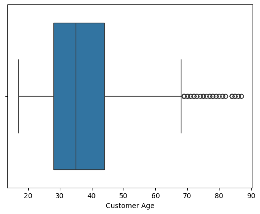
We can see that there are some outliers, but not many. The interquartile range (IQR) is between 29 and 44 years old, with a minimum of 15 and a maximum of 68. There are a few outliers outside the max, but not too many to cause concern.
Let's look at the revenue column next.
sns.boxplot(data=db, x='Revenue')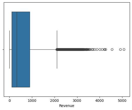
Q1 = db['Revenue'].quantile(0.25)
Q3 = db['Revenue'].quantile(0.75)
IQR = Q3 - Q1

outliers = db[(db['Revenue'] < Q1 - 1.5 * IQR) | (db['Revenue'] > Q3 + 1.5 * IQR)]
print("Number of outliers in Revenue:", len(outliers))Number of outliers in Revenue: 2801
Revenue seems to have many outliers, which makes sense. Purchases can vary greatly in price, and individual's incomes can have big ranges.
Let's take a look at the number of countries present to see if that correlates to real world numbers.
print(db['Country'].nunique())

print(db['Country'].unique())4 ['United States' 'France' 'United Kingdom' 'Germany' nan]
We can see that there are only 4 countries in the dataset, which is not very realistic. Our result will be biased towards developed NA / EU countries. Unfortunately, this is the highest quality free dataset I could find, so we will have to work with it.
Data Preprocessing
After EDA, we can start to preprocess the data. This is the process of cleaning and transforming the data to make it suitable for modeling. The goal is to prepare the data so that it can be used to train a model. This consists of cleaning the data (using the information gathered in EDA step), and feature engineering.
First, we need to clean the data. This involves removing any unnecessary columns, handling missing values, and converting data types. If you are following along, I created a new file called '02_preprocessing.ipynb' in the notebooks folder.
Let's import the data and take a look at it again.
import pandas as pd

db = pd.read_csv("../data/raw/SalesForCourse_quizz_table.csv")
db.head()index Date Year Month Customer Age Customer Gender Country State Product Category Sub Category Quantity Unit Cost Unit Price Cost Revenue Column1 0 0 02/19/16 2016.0 February 29.0 F United States Washington Accessories Tires and Tubes 1.0 80.00 109.000000 80.0 109.0 NaN 1 1 02/20/16 2016.0 February 29.0 F United States Washington Clothing Gloves 2.0 24.50 28.500000 49.0 57.0 NaN 2 2 02/27/16 2016.0 February 29.0 F United States Washington Accessories Tires and Tubes 3.0 3.67 5.000000 11.0 15.0 NaN 3 3 03/12/16 2016.0 March 29.0 F United States Washington Accessories Tires and Tubes 2.0 87.50 116.500000 175.0 233.0 NaN 4 4 03/12/16 2016.0 March 29.0 F United States Washington Accessories Tires and Tubes 3.0 35.00 41.666667 105.0 125.0 NaN
We can see that the data is the same as before. From the EDA step, we know that the 'Column1' column is not needed, as it has no useful information. Let's remove the 'Column1' column, as it is not needed.
print("Missing values before:
", db.isnull().sum())
db.drop(columns=['Column1'], inplace=True)
db.dropna(inplace=True)
print("
Missing values after:
", db.isnull().sum())Missing values before: index 0 Date 1 Year 1 Month 1 Customer Age 1 Customer Gender 1 Country 1 State 1 Product Category 1 Sub Category 1 Quantity 1 Unit Cost 1 Unit Price 1 Cost 1 Revenue 0 Column1 32293 dtype: int64 Missing values after: index 0 Date 0 Year 0 Month 0 Customer Age 0 Customer Gender 0 Country 0 State 0 Product Category 0 Sub Category 0 Quantity 0 Unit Cost 0 Unit Price 0 Cost 0 Revenue 0 dtype: int64
Our data no longer has any missing values, and the 'Column1' column has been removed.
Let's convert dates to datetime objects.
db['Date'] = pd.to_datetime(db['Date'])Make sure strings are formatted correctly.
db['Customer Gender'] = db['Customer Gender'].str.lower().str.strip()
db['Country'] = db['Country'].str.strip()
db['State'] = db['State'].str.strip()
db['Product Category'] = db['Product Category'].str.strip()
db['Sub Category'] = db['Sub Category'].str.strip()
Some values in our data can be unrealistic, so lets remove them. I will limit ages to between 0 and 120, and revenue values to above 0.
db = db[(db['Customer Age'] >= 0) & (db['Customer Age'] <= 120)]
db = db[db['Revenue'] >= 0]
Finally, remove the index column. It can mess with our data and is not relevant.
db = db.drop(columns=['index'])Now that the data is cleaned, we can start feature engineering. Feature engineering is the process of creating new features from existing ones to improve the model's performance. This can include creating new columns, transforming existing columns, and combining multiple columns.
Some datapoints that might be useful could be the year and month of sale, for a general timeframe. Also, the day of the week could be useful, as I think more purchases occur on the weekend. Also, since the dataset includes both unit cost and unit price, I can calculate the profit margin for each sale. Perhaps items with higher profit margins tend to be bought less, and affect revenue. I will create a new column for each of these, and since I will now have the year, month, and day of week, I can drop the 'Date' column.
db['Year'] = db['Date'].dt.year
db['Month'] = db['Date'].dt.month
db['DayOfWeek'] = db['Date'].dt.dayofweek
db['Profit Margin'] = db['Unit Price'] - db['Unit Cost']

db = db.drop(columns=['Date'])
Finally, we can view the processed data.
db.head()Year Month Customer Age Customer Gender Country State Product Category Sub Category Quantity Unit Cost Unit Price Cost Revenue DayOfWeek Profit Margin 0 2016 2 29.0 f United States Washington Accessories Tires and Tubes 1.0 80.00 109.000000 80.0 109.0 4 29.000000 1 2016 2 29.0 f United States Washington Clothing Gloves 2.0 24.50 28.500000 49.0 57.0 5 4.000000 2 2016 2 29.0 f United States Washington Accessories Tires and Tubes 3.0 3.67 5.000000 11.0 15.0 5 1.330000 3 2016 3 29.0 f United States Washington Accessories Tires and Tubes 2.0 87.50 116.500000 175.0 233.0 5 29.000000 4 2016 3 29.0 f United States Washington Accessories Tires and Tubes 3.0 35.00 41.666667 105.0 125.0 5 6.666667
We can see that the data is now cleaned and has new features. The data is now ready for modeling. Let's save our data in the data/processed folder.
db.to_csv("../data/processed/SalesForCourse_processed.csv", index=False)It is fine to use Jupiter Notebooks for preprocessing for a first time to see each output and change, but it is reccommended to use a script to replicate this step if needed in the future. You can find my script in the repo in src folder, namede 'preprocess.py'.
Model Creation
We will use a premade SciKit machine learning model called 'Linear Regression'. It is a common model used in Statistics to explain the relationships between variables. It is a good simple model to use for our first time, and it is easy to understand. The explanitory/independent variables (IV) will be used to train the model on how they affect the dependent variable (DV), which is is what we are predicting (revenue in our case).
Linear regression is a supervised learning algorithm, meaning it uses labeled data that has known categories or values to which it belongs to. This is stronger in most instances than unsupervised learning, which uses unlabeled data to find patterns and relationships in the data, but getting supervised data is much harder. Other common supervised learning algorithms include Decision Trees, Random Forests, and Support Vector Machines. Common unsupervised learning algorithms include clustering, dimensionality reduction, and association rule learning.
We could manually code out the model ourselves, but there is no point when open-source well-documented libraries exist for this.
I created a new file called '03_modeling.ipynb' in the notebooks folder. Let's import the data and take a look at it again.
import pandas as pd
db = pd.read_csv("../data/processed/cleaned_data.csv")
We will now define our target / IV (what we want to predict, revenue in our case), and features / DV (what is used to predict the target).
x = db.drop(columns=["Revenue"])
y = db['Revenue']
X represents our features / input. Y represents our target / output.
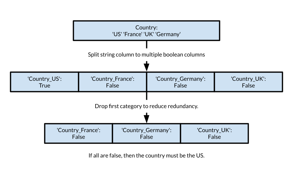
The model of course doesn't understand words/strings, so we must encode them into numbers. Each categorical column is replaced by multiple new boolean cols, one per category (dummy variables). If the string column has 4 categories, it will be split into 4 new columns of each country. Then, one is dropped to avoid the dummy variable trap, which is when one of the columns can be derived from the others, and thus is redundant.
print("X without dummies:")
print(x.head())

x = pd.get_dummies(x, drop_first=True)

print("\n\n\nX with dummies:")
print(x.head())X without dummies: Year Month Customer Age Customer Gender Country State 0 2016 2 29.0 f United States Washington 1 2016 2 29.0 f United States Washington 2 2016 2 29.0 f United States Washington 3 2016 3 29.0 f United States Washington 4 2016 3 29.0 f United States Washington Product Category Sub Category Quantity Unit Cost Unit Price Cost 0 Accessories Tires and Tubes 1.0 80.00 109.000000 80.0 1 Clothing Gloves 2.0 24.50 28.500000 49.0 2 Accessories Tires and Tubes 3.0 3.67 5.000000 11.0 3 Accessories Tires and Tubes 2.0 87.50 116.500000 175.0 4 Accessories Tires and Tubes 3.0 35.00 41.666667 105.0 DayOfWeek Profit Margin 0 4 29.000000 1 5 4.000000 2 5 1.330000 3 5 29.000000 4 5 6.666667 X with dummies: Year Month Customer Age Quantity Unit Cost Unit Price Cost 0 2016 2 29.0 1.0 80.00 109.000000 80.0 1 2016 2 29.0 2.0 24.50 28.500000 49.0 2 2016 2 29.0 3.0 3.67 5.000000 11.0 3 2016 3 29.0 2.0 87.50 116.500000 175.0 4 2016 3 29.0 3.0 35.00 41.666667 105.0 DayOfWeek Profit Margin Customer Gender_m ... Sub Category_Helmets 0 4 29.000000 False ... False 1 5 4.000000 False ... False 2 5 1.330000 False ... False 3 5 29.000000 False ... False 4 5 6.666667 False ... False Sub Category_Hydration Packs Sub Category_Jerseys 0 False False 1 False False 2 False False 3 False False 4 False False Sub Category_Mountain Bikes Sub Category_Road Bikes Sub Category_Shorts 0 False False False 1 False False False 2 False False False 3 False False False 4 False False False Sub Category_Socks Sub Category_Tires and Tubes 0 False True 1 False False 2 False True 3 False True 4 False True Sub Category_Touring Bikes Sub Category_Vests 0 False False 1 False False 2 False False 3 False False 4 False False [5 rows x 75 columns]
(Output is cutoff as there are many categories, but you can see the difference).
print(x.columns.tolist())['Year', 'Month', 'Customer Age', 'Quantity', 'Unit Cost', 'Unit Price', 'Cost', 'DayOfWeek', 'Profit Margin', 'Customer Gender_m', 'Country_Germany', 'Country_United Kingdom', 'Country_United States', 'State_Arizona', 'State_Bayern', 'State_Brandenburg', 'State_California', 'State_Charente-Maritime', 'State_England', 'State_Essonne', 'State_Florida', 'State_Garonne (Haute)', 'State_Georgia', 'State_Hamburg', 'State_Hauts de Seine', 'State_Hessen', 'State_Illinois', 'State_Kentucky', 'State_Loir et Cher', 'State_Loiret', 'State_Massachusetts', 'State_Minnesota', 'State_Mississippi', 'State_Missouri', 'State_Montana', 'State_Moselle', 'State_New York', 'State_Nord', 'State_Nordrhein-Westfalen', 'State_North Carolina', 'State_Ohio', 'State_Oregon', 'State_Pas de Calais', 'State_Saarland', 'State_Seine (Paris)', 'State_Seine Saint Denis', 'State_Seine et Marne', 'State_Somme', 'State_South Carolina', 'State_Texas', 'State_Utah', "State_Val d'Oise", 'State_Val de Marne', 'State_Virginia', 'State_Washington', 'State_Wyoming', 'State_Yveline', 'Product Category_Bikes', 'Product Category_Clothing', 'Sub Category_Bike Stands', 'Sub Category_Bottles and Cages', 'Sub Category_Caps', 'Sub Category_Cleaners', 'Sub Category_Fenders', 'Sub Category_Gloves', 'Sub Category_Helmets', 'Sub Category_Hydration Packs', 'Sub Category_Jerseys', 'Sub Category_Mountain Bikes', 'Sub Category_Road Bikes', 'Sub Category_Shorts', 'Sub Category_Socks', 'Sub Category_Tires and Tubes', 'Sub Category_Touring Bikes', 'Sub Category_Vests']
We now need to split the data. Why? We can't test the model on the data it trained on, as it would already know the answer, so we exclude some data from the training data to be used for testing later.
We set aside 20% of the data for testing, and use the rest for training. This is a common practice in machine learning.
from sklearn.model_selection import train_test_split

x_train, x_test, y_train, y_test = train_test_split(
    x, y, test_size=0.2, random_state=42
)
Now comes the training part. ScikitLearn makes this very easy to do, just import the model, specify which we use, and fit it to the feature and target dataframes.
from sklearn.linear_model import LinearRegression
model = LinearRegression()
model.fit(x_train, y_train)
So, is it good, or even working? Let's evaluate using our testing data.
from sklearn.metrics import mean_absolute_error, mean_squared_error, r2_score

y_pred = model.predict(x_test)

print("MAE:", mean_absolute_error(y_test, y_pred))
print("RMSE:", pd.Series(mean_squared_error(y_test, y_pred)).pow(0.5).iloc[0])
print("R2 Score:", r2_score(y_test, y_pred))MAE: 34.50387929187516 RMSE: 60.661287924114156 R2 Score: 0.9932158085795341
Let's interpret the results:
- MAE (Mean Absolute Error): Mean away from true value. Lower is better. We are $33.50 off of the real value on average.
- RMSE (Root Mean Squared Error): Similar to MAE but penalizes big errors more (it squares them before averaging). So a few really bad predictions can maek RMSE goes up faster than MAE. Our RSME is $60.66.
- R2 (R-Squared Score): How well the model explains the variance in the data. 0 explains none of the variance, 0.99 explains 99% of the variance, adn 1 explains 100% of the variance. Ours is 0.9932.
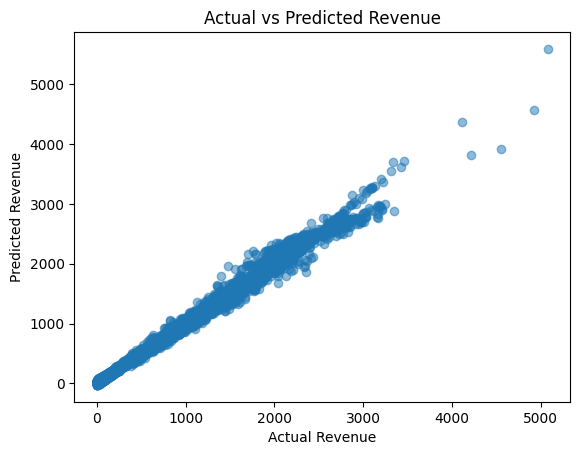
We can also look at a scatterplot to determine our model's success. The closer to a diagonal, the better.

Our model can be assessed are accurate. Our R2 is very close to 1, the MAE is small compared to average values, and the scatterplot shows that our predictions are close to the actual values.
Finally, let's save our model.
import os
import joblib

os.makedirs('models', exist_ok=True)
joblib.dump(model, '../models/model.pkl')
print("Model saved to models/model.pkl")
As with our preprocessing step, it is a good idea to create a script that can be run to replicate the model training step. You can find my script in the repo in src folder, named 'train.py'.
Results
Now that we have a working model, let's see what it will predict with random data. I created a new notebook called '04_results.ipynb' for this.
import pandas as pd
import numpy as np
import joblib
import random

feature_cols = [
    'Year', 'Month', 'Customer Age', 'Quantity', 'Unit Cost', 'Unit Price', 'Cost', 'DayOfWeek', 'Profit Margin',
    'Customer Gender_m', 'Country_Germany', 'Country_United Kingdom', 'Country_United States',
    'State_Arizona', 'State_Bayern', 'State_Brandenburg', 'State_California', 'State_Charente-Maritime',
    'State_England', 'State_Essonne', 'State_Florida', 'State_Garonne (Haute)', 'State_Georgia',
    'State_Hamburg', 'State_Hauts de Seine', 'State_Hessen', 'State_Illinois', 'State_Kentucky',
    'State_Loir et Cher', 'State_Loiret', 'State_Massachusetts', 'State_Minnesota', 'State_Mississippi',
    'State_Missouri', 'State_Montana', 'State_Moselle', 'State_New York', 'State_Nord',
    'State_Nordrhein-Westfalen', 'State_North Carolina', 'State_Ohio', 'State_Oregon',
    'State_Pas de Calais', 'State_Saarland', 'State_Seine (Paris)', 'State_Seine Saint Denis',
    'State_Seine et Marne', 'State_Somme', 'State_South Carolina', 'State_Texas', 'State_Utah',
    "State_Val d'Oise", 'State_Val de Marne', 'State_Virginia', 'State_Washington', 'State_Wyoming',
    'State_Yveline', 'Product Category_Bikes', 'Product Category_Clothing', 'Sub Category_Bike Stands',
    'Sub Category_Bottles and Cages', 'Sub Category_Caps', 'Sub Category_Cleaners', 'Sub Category_Fenders',
    'Sub Category_Gloves', 'Sub Category_Helmets', 'Sub Category_Hydration Packs', 'Sub Category_Jerseys',
    'Sub Category_Mountain Bikes', 'Sub Category_Road Bikes', 'Sub Category_Shorts', 'Sub Category_Socks',
    'Sub Category_Tires and Tubes', 'Sub Category_Touring Bikes', 'Sub Category_Vests'
]

n_samples = 10

# Initialize with zeros
sample_data = pd.DataFrame(0, index=np.arange(n_samples), columns=feature_cols)


# Group columns by category prefix for random selection
gender_cols = ['Customer Gender_m']  # binary example; assuming 'm' means male (1) or female (0)
country_cols = ['Country_Germany', 'Country_United Kingdom', 'Country_United States']
state_cols = [col for col in feature_cols if col.startswith('State_')]
product_category_cols = ['Product Category_Bikes', 'Product Category_Clothing']
sub_category_cols = [col for col in feature_cols if col.startswith('Sub Category_')]

# Helper function to create zero vectors and set one randomly to 1
def one_hot_random(cols, n_samples):
    arr = np.zeros((n_samples, len(cols)), dtype=int)
    for i in range(n_samples):
        idx = random.randint(0, len(cols) - 1)
        arr[i, idx] = 1
    return pd.DataFrame(arr, columns=cols)
Run the block below to generate sample data.
n_samples = 10

# Create numeric features with fixed or random values
sample_data = pd.DataFrame({
    'Year': [2023]*n_samples,
    'Month': [random.randint(1, 12) for _ in range(n_samples)],
    'Customer Age': [random.randint(18, 65) for _ in range(n_samples)],
    'Quantity': [random.randint(1, 5) for _ in range(n_samples)],
    'Unit Cost': [round(random.uniform(10, 100), 2) for _ in range(n_samples)],
    'Unit Price': [round(random.uniform(20, 150), 2) for _ in range(n_samples)],
    'Cost': 0,  # will calculate next
    'DayOfWeek': [random.randint(0, 6) for _ in range(n_samples)],
    'Profit Margin': 0,  # will calculate next
})

# Calculate Cost and Profit Margin
sample_data['Cost'] = sample_data['Quantity'] * sample_data['Unit Cost']
sample_data['Profit Margin'] = sample_data['Unit Price'] - sample_data['Unit Cost']

# Generate random one-hot for categorical columns
sample_gender = one_hot_random(gender_cols, n_samples)
sample_country = one_hot_random(country_cols, n_samples)
sample_state = one_hot_random(state_cols, n_samples)
sample_product_category = one_hot_random(product_category_cols, n_samples)
sample_sub_category = one_hot_random(sub_category_cols, n_samples)

# Combine all into one DataFrame
sample_data = pd.concat([sample_data,
                         sample_gender,
                         sample_country,
                         sample_state,
                         sample_product_category,
                         sample_sub_category], axis=1)

# Make sure columns order matches model expectation
sample_data = sample_data[feature_cols]
Run the block below to see the results.
model = joblib.load('../models/model.pkl')

predictions = model.predict(sample_data)

for i in range(len(sample_data)):
    row = sample_data.iloc[i]
    # Extract key details
    year = row['Year']
    month = row['Month']
    age = row['Customer Age']
    quantity = row['Quantity']
    unit_price = row['Unit Price']
    day_of_week = row['DayOfWeek']

    # Find which gender, country, state, product category, subcategory is set to 1
    gender = 'Male' if row['Customer Gender_m'] == 1 else 'Female'

    # For countries (only one should be 1)
    countries = ['Germany', 'United Kingdom', 'United States']
    country_cols = ['Country_Germany', 'Country_United Kingdom', 'Country_United States']
    country = [c for c, col in zip(countries, country_cols) if row[col] == 1]
    country = country[0] if country else 'Unknown'

    # States
    state_cols = [col for col in sample_data.columns if col.startswith('State_')]
    state = [col.replace('State_', '') for col in state_cols if row[col] == 1]
    state = state[0] if state else 'Unknown'

    # Product Category
    product_categories = ['Bikes', 'Clothing']
    product_cols = ['Product Category_Bikes', 'Product Category_Clothing']
    product_category = [p for p, col in zip(product_categories, product_cols) if row[col] == 1]
    product_category = product_category[0] if product_category else 'Unknown'

    # Sub Category (multiple, but presumably only one is 1)
    sub_cat_cols = [col for col in sample_data.columns if col.startswith('Sub Category_')]
    sub_category = [col.replace('Sub Category_', '') for col in sub_cat_cols if row[col] == 1]
    sub_category = sub_category[0] if sub_category else 'Unknown'

    print(f"Sample {i+1}: Year={year}, Month={month}, Age={age}, Quantity={quantity}, Unit Price=${unit_price:.2f}, "
          f"DayOfWeek={day_of_week}, Gender={gender}, Country={country}, State={state}, "
          f"Product Category={product_category}, Sub Category={sub_category}")
    print(f"  Predicted Revenue: ${predictions[i]:.2f}
")
Sample 1: Year=2023.0, Month=6.0, Age=34.0, Quantity=3.0, Unit Price=$109.93, DayOfWeek=1.0, Gender=Male, Country=Germany, State=Yveline, Product Category=Bikes, Sub Category=Jerseys
  Predicted Revenue: $447.85

Sample 2: Year=2023.0, Month=3.0, Age=21.0, Quantity=5.0, Unit Price=$67.18, DayOfWeek=2.0, Gender=Male, Country=United Kingdom, State=Texas, Product Category=Clothing, Sub Category=Mountain Bikes
  Predicted Revenue: $570.25

Sample 3: Year=2023.0, Month=10.0, Age=44.0, Quantity=4.0, Unit Price=$44.36, DayOfWeek=2.0, Gender=Male, Country=United Kingdom, State=Bayern, Product Category=Bikes, Sub Category=Touring Bikes
  Predicted Revenue: $521.61

Sample 4: Year=2023.0, Month=12.0, Age=36.0, Quantity=4.0, Unit Price=$23.38, DayOfWeek=2.0, Gender=Male, Country=United States, State=Washington, Product Category=Bikes, Sub Category=Bike Stands
  Predicted Revenue: $310.69

Sample 5: Year=2023.0, Month=3.0, Age=27.0, Quantity=2.0, Unit Price=$128.36, DayOfWeek=6.0, Gender=Male, Country=United Kingdom, State=Arizona, Product Category=Bikes, Sub Category=Vests
  Predicted Revenue: $428.41

Sample 6: Year=2023.0, Month=12.0, Age=25.0, Quantity=2.0, Unit Price=$136.36, DayOfWeek=2.0, Gender=Male, Country=United Kingdom, State=Seine et Marne, Product Category=Clothing, Sub Category=Vests
  Predicted Revenue: $440.49

Sample 7: Year=2023.0, Month=4.0, Age=38.0, Quantity=1.0, Unit Price=$71.26, DayOfWeek=2.0, Gender=Male, Country=Germany, State=Texas, Product Category=Clothing, Sub Category=Cleaners
  Predicted Revenue: $268.86

Sample 8: Year=2023.0, Month=5.0, Age=38.0, Quantity=1.0, Unit Price=$112.11, DayOfWeek=1.0, Gender=Male, Country=Germany, State=Hamburg, Product Category=Clothing, Sub Category=Bottles and Cages
  Predicted Revenue: $318.19

Sample 9: Year=2023.0, Month=4.0, Age=44.0, Quantity=1.0, Unit Price=$139.08, DayOfWeek=1.0, Gender=Male, Country=United Kingdom, State=Hauts de Seine, Product Category=Bikes, Sub Category=Tires and Tubes
  Predicted Revenue: $302.11

Sample 10: Year=2023.0, Month=11.0, Age=24.0, Quantity=3.0, Unit Price=$57.38, DayOfWeek=5.0, Gender=Male, Country=Germany, State=Kentucky, Product Category=Clothing, Sub Category=Vests
  Predicted Revenue: $491.76